LFD Workshop FLIM Tutorial#
The LFD Workshop FLIM tutorial adapted to PhasorPy.
This tutorial is a close adaptation of the LFD Workshop computer training tutorial - FLIM section (by E. Gratton, M. Digman, and J. Unruh) using the PhasorPy library instead of the Globals for Images · SimFCS and Excel software.
Note
This tutorial is work in progress. Not all of SimFCS’ functionality is available in the PhasorPy library yet.
Import required modules and functions:
import numpy
from matplotlib import pyplot

from phasorpy.datasets import fetch
from phasorpy.io import phasor_from_simfcs_referenced
from phasorpy.phasor import (
    lifetime_fraction_from_amplitude,
    lifetime_to_signal,
    phasor_filter,
    phasor_from_fret_donor,
    phasor_from_lifetime,
    phasor_threshold,
    phasor_to_apparent_lifetime,
    phasor_to_polar,
)
from phasorpy.plot import (
    PhasorPlot,
    plot_phasor,
    plot_phasor_image,
    plot_polar_frequency,
)
Phasor properties#
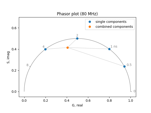
The phasor is a frequency domain representation of the fluorescence lifetime at a single frequency. For single exponential lifetimes, this completely describes the system. For multiple exponentials, the phasor represents some intensity weighted linear combination of the lifetimes in the system. Therefore, given the phasor for a single multiexponential measurement, we cannot determine the lifetimes for the system. Nevertheless, given multiple measurements (e.g. multiple pixels in an image), heterogeneity becomes obvious.
To demonstrate this effect, calculate:
the phasor at a single frequency for a combination of four exponentials:
frequency = 80.0  # MHz
lifetimes = [4.0, 2.0, 1.0, 0.5]  # ns
amplitudes = [0.25, 0.25, 0.25, 0.25]  # pre-exponential amplitudes

phasor_single = phasor_from_lifetime(frequency, lifetimes)
phasor_combined = phasor_from_lifetime(
    frequency, lifetimes, amplitudes, preexponential=True
)

plot = PhasorPlot(frequency=frequency)
plot.components(
    *phasor_single, lifetime_fraction_from_amplitude(lifetimes, amplitudes)
)
plot.plot(*phasor_single, label='single components')
plot.plot(*phasor_combined, label='combined components')
plot.show()
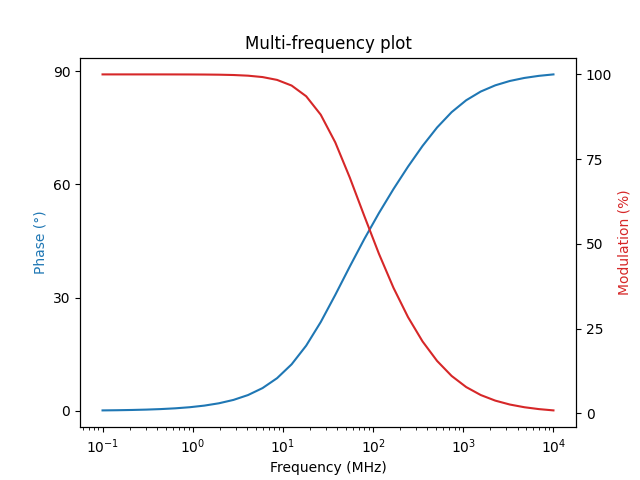
the multi-frequency fluorescence modulation and phase curves:
frequencies = numpy.logspace(-1, 4, 32)

phase, modulation = phasor_to_polar(
    *phasor_from_lifetime(
        frequencies, lifetimes, amplitudes, preexponential=True
    )
)

plot_polar_frequency(frequencies, phase, modulation)
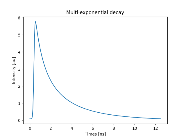
the time-domain fluorescence decay:
signal, instrument_response, times = lifetime_to_signal(
    frequency, lifetimes, amplitudes, preexponential=True, samples=256
)

fig, ax = pyplot.subplots()
ax.set(
    title='Multi-exponential decay',
    xlabel='Times [ns]',
    ylabel='Intensity [au]',
)
ax.plot(times, signal)
pyplot.show()
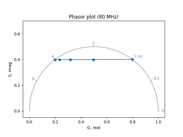
Two state equilibrium#
Fluorescent ion indicators often exist in two distinct states with different emission spectra and fluorescence lifetimes (and sometimes absorption spectra). The lifetime may be multiexponential in both the free and ion-bound state. Binding to the ion of interest shifts the equilibrium between these states, changing the spectral properties and the fluorescence lifetimes. Therefore, the free and bound states will be characterized by different “phasors”. Close to the dissociation constant, the fluorescence lifetime is characterized by a linear combination of the two phasors.
Simulate the phasor for different combinations (relative amplitudes) of a 4 ns lifetime state and a 1 ns lifetime state (e.g. amplitude 1 = 0.2, amplitude 2 = 0.8).
frequency = 80.0  # MHz
lifetimes = [4.0, 1.0]  # ns
amplitudes_list = [[1.0, 0.0], [0.8, 0.2], [0.5, 0.5], [0.2, 0.8], [0.0, 1.0]]

real, imag = phasor_from_lifetime(
    frequency, lifetimes, amplitudes_list, preexponential=True
)
Record S (the phasor y coordinate) and G (the phasor x coordinate) values for each combination.
print('S:', imag)
print('G:', real)
S: [0.3987275  0.39887702 0.39923587 0.39999843 0.40126936]
G: [0.19831079 0.23360427 0.31830864 0.49830541 0.79830002]
Plot S vs. G to see how the phasor changes with different combinations.
plot_phasor(real, imag, fmt='o-', frequency=frequency)
Questions:
When half of the population is in the 1 ns state, has the phasor moved halfway between the phasors for the two states?
Does the position of the phasor change linearly with concentration?
What about with fractional intensity?
What information is needed to calculate concentration from the position of a phasor?
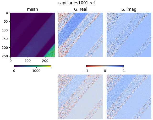
Capillaries#
The file, capillaries1001.ref, contains phase and modulation data on
three capillaries filled with different dye solutions.
The extension .ref, for referenced, indicates that this file has been
corrected for phase shifts and detection efficiency relative to a reference
with a known lifetime (e.g., Fluorescein).
Read the file, calculate phasor coordinates from phase and modulation,
display the images, and plot the phasor coordinates of first and second
harmonics:
frequency = 80.0  # MHz
mean, real, imag = phasor_from_simfcs_referenced(
    fetch('capillaries1001.ref'), harmonic=[1, 2]
)
real1, real2 = real
imag1, imag2 = imag
plot_phasor_image(mean, real, imag, title='capillaries1001.ref')
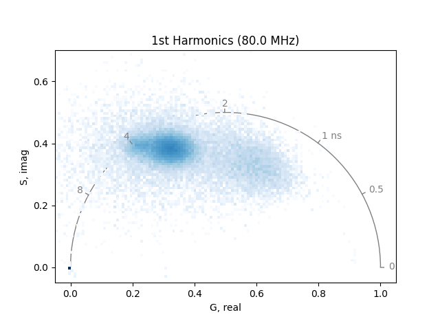
plot_phasor(
    real1,
    imag1,
    frequency=frequency,
    style='hist2d',
    cmin=4,
    title=f'1st Harmonics ({frequency} MHz)',
)
plot_phasor(
    real2,
    imag2,
    frequency=frequency * 2,
    style='hist2d',
    cmin=4,
    title=f'2nd Harmonics ({frequency * 2} MHz)',
)
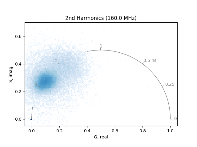
The two phasor plots show the pixel phasor distribution for the first and second harmonics (for the two-photon systems these would be 80 MHz and 160 MHz).
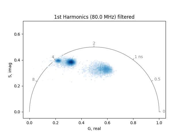
The calculation of the phase and modulation is strongly dependent on the signal-to-noise. Therefore, it is a good idea to smooth noisy data by a moving average. Note that this will also reduce the spatial resolution in the phasor.
If high spatial resolution is needed, make sure to have at least 100 photons in each pixel of the image.
real1, imag1 = phasor_filter(real1, imag1, method='median', repeat=2)
real2, imag2 = phasor_filter(real2, imag2, method='median', repeat=2)
In addition, small amounts of room light will appear towards the lower left-hand corner of the phasor (room light is uncorrelated, so it has zero modulation depth). This can be eliminated by setting a threshold.
_, real1, imag1 = phasor_threshold(
    mean, real1, imag1, mean_min=20, real_min=0, imag_min=0, open_interval=True
)
_, real2, imag2 = phasor_threshold(
    mean, real2, imag2, mean_min=20, real_min=0, imag_min=0, open_interval=True
)
plot_phasor(
    real1,
    imag1,
    frequency=frequency,
    style='hist2d',
    cmin=4,
    title=f'1st Harmonics ({frequency} MHz) filtered',
)
plot_phasor(
    real2,
    imag2,
    frequency=frequency * 2,
    style='hist2d',
    cmin=4,
    title=f'2nd Harmonics ({frequency * 2} MHz) filtered',
)
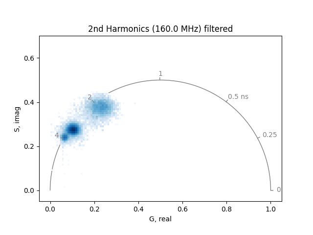
Note that if the room light is significant compared to the fluorescence signal, it will bias the fluorescence phasors by pulling them toward the lower left-hand corner of the phasor plot, with phasors corresponding to lower intensity regions of the image being pulled more toward the lower left-hand corner than those of higher intensity regions of the image.
Todo
Select different components of the phasor using cursors. List the phase and modulation well as the apparent phase and modulation lifetimes for the selected components.
All of the capillaries contain 10 mM Tris buffer, pH 8.0. Fluorescein has a lifetime of 4.05 ns in basic solution.
Which capillary contains Fluorescein?
The shortest lifetime capillary contains Rhodamine B, which has a single exponential lifetime around 1.5 ns in phosphate buffer at pH 7.0.
Is Rhodamine B single exponential in this solution?
What does the center capillary contain?
Todo
The phasor cursors can be assigned different colors. This allows to have different phasor distributions displayed simultaneously.
Todo
Move a green cursor around the phasor space to highlight the pixels in the image that correspond to a specific phasor distribution.
Todo
Another feature is the mapping (linking) of the linear combination (fractional intensity) of two different lifetime signatures associated with two different species.
Link the red and green cursors.
Todo
To visualize the linear combination of the two colors (species):
Place the 2 cursors on the part of the image to link and show the linked cursor bitmap for harmonic 1.
The color bitmap shows the relative concentration of the selected species.
The explanations in the last two paragraphs should help answer the last question above, about the components in the middle channel.
Quenching, FRET#
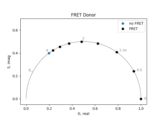
This section will discuss quenching due to FRET. The efficiency of energy transfer is related to the fluorescence lifetime as follows:
where \(\tau_{DA}\) is the lifetime of the donor in the presence of acceptor (quenched) and \(\tau_{D}\) is the lifetime of the donor in the absence of acceptor.
Calculate the phasor for a fluorophore with a 4 ns lifetime. Then calculate its phasor under different efficiencies of energy transfer. How does this differ from what we saw with the two-state system?
plot = PhasorPlot(frequency=frequency, title='FRET Donor')
plot.plot(*phasor_from_lifetime(frequency, lifetime=4.0), label='no FRET')
plot.plot(
    *phasor_from_lifetime(frequency, 4.0 * (1 - numpy.linspace(0.1, 1.0, 8))),
    color='k',
    label='FRET',
)
plot.show()
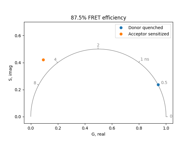
If only the donor fluorophore is excited (no direct excitation of the acceptor), the acceptor fluorescence shows a very unusual phenomenon. The fluorescence of the acceptor rises with the same time constant as the quenched donor fluorescence. Then it decays with the characteristic lifetime of the acceptor. For example, when the donor lifetime has been quenched to 0.5 ns and the acceptor lifetime is 4 ns, the acceptor can be simulated by a lifetime of 0.5 ns with amplitude of -1 and a lifetime of 4 ns with amplitude of 1:
plot = PhasorPlot(frequency=frequency, title='87.5% FRET efficiency')
plot.plot(
    *phasor_from_lifetime(frequency, lifetime=0.5), label='Donor quenched'
)
plot.plot(
    *phasor_from_lifetime(
        frequency,
        lifetime=[4.0, 0.5],
        fraction=[1.0, -1.0],
        preexponential=True,
    ),
    label='Acceptor sensitized',
)
plot.show()
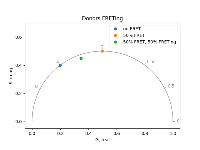
Often in FRET experiments, only a fraction of the donor molecules experience FRET. The others continue to fluoresce with an unquenched lifetime. Simulate the situation where 50% of the donors remain unquenched. Rationalize the results in terms of the quenching simulations done above and the two state experiments we did earlier.
plot = PhasorPlot(frequency=frequency, title='Donors FRETing')
plot.plot(*phasor_from_lifetime(frequency, lifetime=4.0), label='no FRET')
plot.plot(*phasor_from_lifetime(frequency, lifetime=2.0), label='50% FRET')
plot.plot(
    *phasor_from_lifetime(frequency, lifetime=[4.0, 2.0], fraction=[0.5, 0.5]),
    label='50% FRET, 50% FRETing',
)
plot.show()
CFP-YFP#
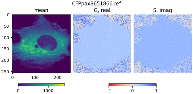
Open the file CFPpax8651866.ref, which contains referenced FLIM data
for a cell transfected with a CFP paxillin construct.
mean1, real1, imag1 = phasor_from_simfcs_referenced(fetch('CFPpax8651866.ref'))

plot_phasor_image(mean1, real1, imag1, title='CFPpax8651866.ref')
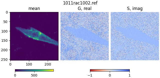
Open the file 1011rac1002.ref, which contains referenced FLIM data
for a cell transfected with a CFP-YFP fusion protein:
mean2, real2, imag2 = phasor_from_simfcs_referenced(fetch('1011rac1002.ref'))

plot_phasor_image(mean2, real2, imag2, title='1011rac1002.ref')
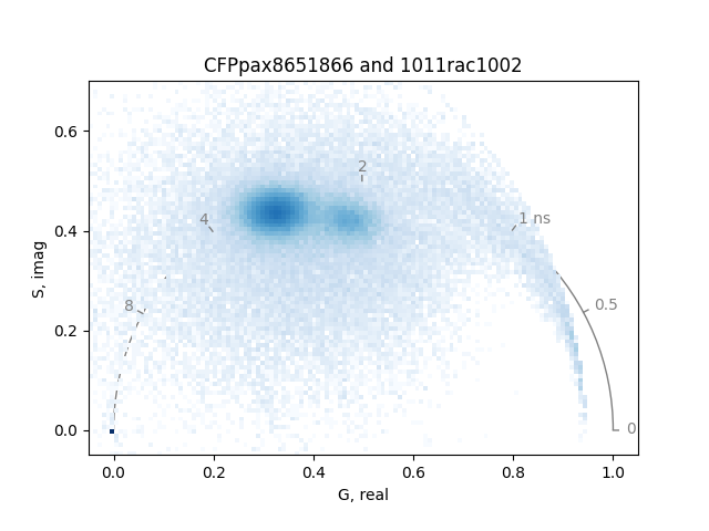
Plot the phasor distributions together:
frequency = 80.0  # MHz

plot = PhasorPlot(frequency=frequency, title='CFPpax8651866 and 1011rac1002')
plot.hist2d([real1, real2], [imag1, imag2], cmap='Blues', cmin=4)
plot.show()
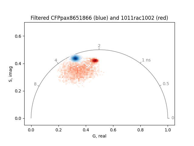
Set the intensity threshold to 32 to remove any room light and smooth the phasor.
real1, imag1 = phasor_filter(real1, imag1, method='median', repeat=2)
real2, imag2 = phasor_filter(real2, imag2, method='median', repeat=2)

_, real1, imag1 = phasor_threshold(
    mean, real1, imag1, mean_min=32, real_min=0, imag_min=0, open_interval=True
)
_, real2, imag2 = phasor_threshold(
    mean, real2, imag2, mean_min=32, real_min=0, imag_min=0, open_interval=True
)

plot = PhasorPlot(
    frequency=frequency,
    title='Filtered CFPpax8651866 (blue) and 1011rac1002 (red)',
)
plot.hist2d(real2, imag2, cmap='Reds', cmin=20)  # label='1011rac1002'
plot.hist2d(real1, imag1, cmap='Blues', cmin=20)  # label='CFPpax8651866'
plot.show()
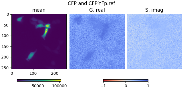
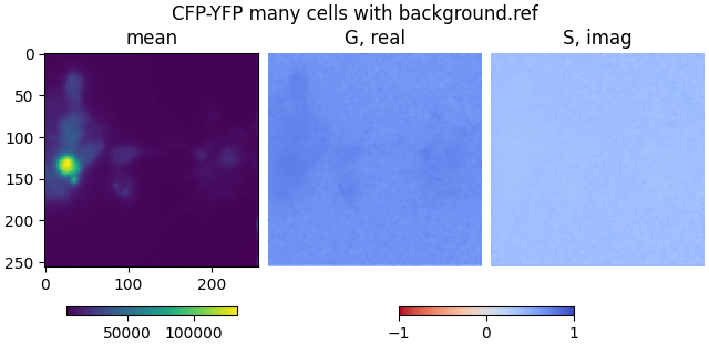
Load CFP and CFP-YFP.ref and CFP-YFP many cells with background.ref.
These files were acquired using the Lambert frequency domain FLIM instrument
and were referenced using a solution of Fluorescein at pH>9.
They contain fixed samples of CFP and CFP-YFP expressing cells with
various amounts of background.
Set the intensity threshold to 6202 counts, such that the background phasor
is visible.
frequency = 80.0  # MHz
mean1, real1, imag1 = phasor_from_simfcs_referenced(
    fetch('CFP and CFP-YFp.ref')
)

plot_phasor_image(mean1, real1, imag1, title='CFP and CFP-YFp.ref')
mean2, real2, imag2 = phasor_from_simfcs_referenced(
    fetch('CFP-YFP many cells with background.ref')
)

plot_phasor_image(
    mean2, real2, imag2, title='CFP-YFP many cells with background.ref'
)
mean = numpy.vstack((mean1, mean2))
real = numpy.vstack((real1, real2))
imag = numpy.vstack((imag1, imag2))

real, imag = phasor_filter(real, imag, method='median', repeat=2)

_, real, imag = phasor_threshold(
    mean, real, imag, mean_min=6202, real_min=0, imag_min=0, open_interval=True
)

plot = PhasorPlot(
    frequency=frequency,
    title='"CFP and CFP-YFp" and "CFP-YFP many cells"',
)
plot.hist2d(real, imag, cmin=1)
plot.show()

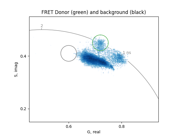
Before starting the analysis of the FRET trajectory, identify the phasor of the donor without the acceptor and the phasor of the background or autofluorescence.
Set two cursors of size 0.03 at the phasor coordinates of the unquenched donor (0.72, 0.45) and the background (0.62, 0.41):
background_phasor = 0.6, 0.41
donor_phasor = 0.72, 0.45
donor_lifetime = numpy.mean(
    phasor_to_apparent_lifetime(*donor_phasor, frequency)
)

plot = PhasorPlot(
    frequency=frequency,
    title='FRET Donor (green) and background (black)',
    xlim=[0.45, 0.94],
    ylim=[0.15, 0.55],
)
plot.hist2d(real, imag)
plot.circle(*donor_phasor, radius=0.03, linestyle='-', color='tab:green')
plot.circle(*background_phasor, radius=0.03, linestyle='-', color='dimgrey')
plot.show()
Calculate two trajectories, one for the quenching due to FRET and the other for the superposition of the FRETing population with the background.
The FRET efficiency for the file with very little background is about 0.23. Instead, the best agreement for the file with large background is obtained with the combination shown below, that results in about 0.32 FRET efficiency.
settings = {
    'frequency': frequency,
    'donor_lifetime': donor_lifetime,
    'donor_freting': 1.0,
    'donor_background': 0.1,
    'background_real': background_phasor[0],
    'background_imag': background_phasor[1],
}

quenching_trajectory = phasor_from_fret_donor(
    **settings, fret_efficiency=numpy.linspace(0.0, 1.0, 100)
)

fret1_phasor = phasor_from_fret_donor(**settings, fret_efficiency=0.23)
fret2_phasor = phasor_from_fret_donor(**settings, fret_efficiency=0.32)

settings['donor_background'] = numpy.linspace(0.0, 100.0, 100)
freting1_trajectory = phasor_from_fret_donor(**settings, fret_efficiency=0.23)
freting2_trajectory = phasor_from_fret_donor(**settings, fret_efficiency=0.32)

plot = PhasorPlot(
    frequency=frequency,
    title='FRET trajectories',
    xlim=[0.45, 0.94],
    ylim=[0.15, 0.55],
)
plot.hist2d(real, imag)
plot.circle(*donor_phasor, radius=0.03, linestyle='-', color='tab:green')
plot.circle(*background_phasor, radius=0.03, linestyle='-', color='dimgrey')
plot.plot(*quenching_trajectory, fmt='-', color='tab:grey')
plot.plot(*freting1_trajectory, fmt='-', color='tab:grey')
plot.plot(*freting2_trajectory, fmt='-', color='tab:grey')
plot.line(
    [background_phasor[0], donor_phasor[0]],
    [background_phasor[1], donor_phasor[1]],
    linestyle='-',
    color='tab:green',
)
plot.plot(*fret1_phasor, color='tab:grey')
plot.plot(*fret2_phasor, color='tab:grey')
plot.show()
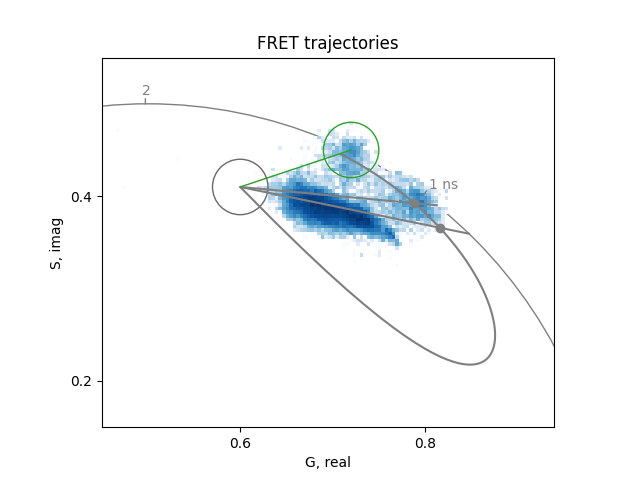
For this sample, it seems that all the cells are FRETing and that the change of lifetime between the cells is due to combination with the background fluorescence.
Todo
Another type of plot that can be obtained is the histogram of the fractional intensity, along the green line, for each file selected.
Assign component 1 and component 2 to the extremes of the lines of the linear combination.
Comments and questions#
There is a large amount of background in some of the files, which is absent in other experiments. This could be due to the media used for fixing the samples. The spatial distribution due to FRET is always obtained at the entire cell level, not internal to a cell since in these samples either a cell expresses one protein of the other.
What percentage of the species is FRETing in the CFP-YFP image?
Is the FRET efficiency high or low?
sphinx_gallery_thumbnail_number = -1 mypy: allow-untyped-defs, allow-untyped-calls mypy: disable-error-code=”arg-type”
Total running time of the script: (0 minutes 4.749 seconds)
Download Jupyter notebook: phasorpy_lfd_workshop.ipynbDownload Python source code: phasorpy_lfd_workshop.pyDownload zipped: phasorpy_lfd_workshop.zipGallery generated by Sphinx-Gallery