Synthesize signals from lifetimes

An introduction to the lifetime_to_signal function.

The phasorpy.phasor.lifetime_to_signal() function is used to synthesize time- and frequency-domain signals as a function of fundamental frequency, single or multiple lifetime components, lifetime fractions, mean and background intensity, and instrument response function (IRF) peak location and width.

Import required modules and functions:

import numpy
from matplotlib import pyplot

from phasorpy.phasor import (
    lifetime_to_signal,
    phasor_calibrate,
    phasor_from_lifetime,
    phasor_from_signal,
)

Define common parameters used throughout the tutorial:

frequency = 80.0  # fundamental frequency in MHz
reference_lifetime = 4.2  # lifetime of reference signal in ns

lifetimes = [0.5, 1.0, 2.0, 4.0]  # lifetime in ns
fractions = [0.25, 0.25, 0.25, 0.25]  # fractional intensities

settings = {
    'samples': 256,  # number of samples to synthesize
    'mean': 1.0,  # average intensity
    'background': 0.0,  # no signal from background
    'zero_phase': None,  # location of IRF peak in the phase
    'zero_stdev': None,  # standard deviation of IRF in radians
}

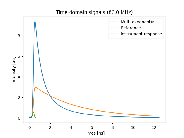
Time-domain, multi-exponential

Synthesize a time-domain signal of a multi-component lifetime system with given fractional intensities, convolved with an instrument response function:

signal, instrument_response, times = lifetime_to_signal(
    frequency, lifetimes, fractions, **settings
)

A reference signal of known lifetime, obtained with the same instrument and sampling parameters, is required to correct/calibrate the phasor coordinates of signals. The calibrated phasor coordinates match the theoretical phasor coordinates expected for the lifetimes:

reference_signal, _, _ = lifetime_to_signal(
    frequency, reference_lifetime, **settings
)


def verify_signal(fractions):
    """Verify calibrated phasor coordinates match expected results."""
    numpy.testing.assert_allclose(
        phasor_calibrate(
            *phasor_from_signal(signal)[1:],
            *phasor_from_signal(reference_signal)[1:],
            frequency,
            reference_lifetime,
        ),
        phasor_from_lifetime(frequency, lifetimes, fractions),
    )


verify_signal(fractions)

Plot the synthesized signal, the instrument response, and reference signal:

fig, ax = pyplot.subplots()
ax.set(
    title=f'Time-domain signals ({frequency} MHz)',
    xlabel='Times [ns]',
    ylabel='Intensity [au]',
)
ax.plot(times, signal, label='Multi-exponential')
ax.plot(times, reference_signal, label='Reference')
ax.plot(times, instrument_response, label='Instrument response')
ax.legend()
pyplot.show()

Time-domain, single-exponential

To synthesize separate signals for each lifetime component at once, omit the lifetime fractions:

signal, _, times = lifetime_to_signal(frequency, lifetimes, **settings)

verify_signal(None)

Plot the synthesized signal:

fig, ax = pyplot.subplots()
ax.set(
    title=f'Time-domain signals ({frequency} MHz)',
    xlabel='Times [ns]',
    ylabel='Intensity [au]',
)
ax.plot(times, signal.T, label=[f'{t} ns' for t in lifetimes])
ax.legend()
pyplot.show()

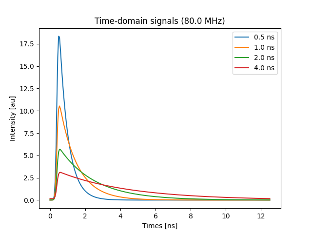
As expected, the shorter the lifetime, the faster the decay.

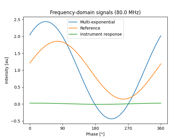
Frequency-domain, multi-exponential

To synthesize a frequency-domain, homodyne signal, limit the synthesis to the fundamental frequency (harmonic=1):

signal, instrument_response, _ = lifetime_to_signal(
    frequency, lifetimes, fractions, harmonic=1, **settings
)

reference_signal, _, _ = lifetime_to_signal(
    frequency, reference_lifetime, harmonic=1, **settings
)

verify_signal(fractions)

Plot the synthesized signals:

phase = numpy.linspace(0.0, 360.0, signal.size)

fig, ax = pyplot.subplots()
ax.set(
    title=f'Frequency-domain signals ({frequency} MHz)',
    xlabel='Phase [°]',
    ylabel='Intensity [au]',
    xticks=[0, 90, 180, 270, 360],
)
ax.plot(phase, signal, label='Multi-exponential')
ax.plot(phase, reference_signal, label='Reference')
ax.plot(phase, instrument_response, label='Instrument response')
ax.legend()
pyplot.show()

Frequency-domain, single-exponential

To synthesize separate signals for each lifetime component at once, omit the lifetime fractions:

signal, _, _ = lifetime_to_signal(frequency, lifetimes, harmonic=1, **settings)

verify_signal(None)

Plot the synthesized signals:

fig, ax = pyplot.subplots()
ax.set(
    title=f'Frequency-domain signals ({frequency} MHz)',
    xlabel='Phase [°]',
    ylabel='Intensity [au]',
    xticks=[0, 90, 180, 270, 360],
)
ax.plot(phase, signal.T, label=[f'{t} ns' for t in lifetimes])
ax.legend()
pyplot.show()

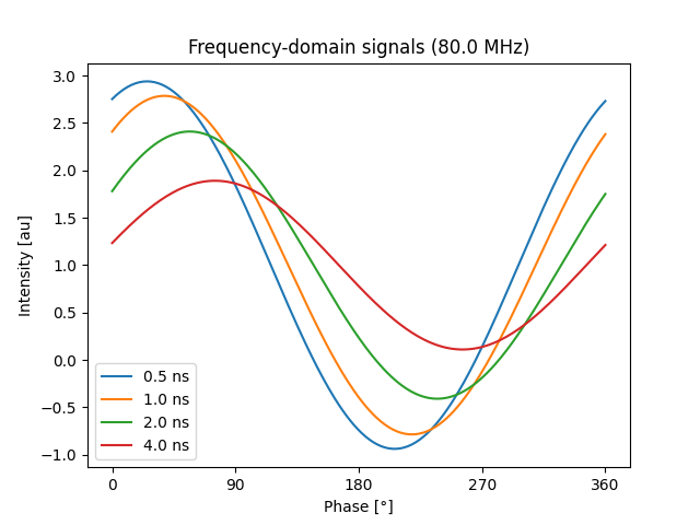
As expected, the shorter the lifetime, the smaller the phase-shift and de-modulation.

TODO: generate digitized image from lifetime distributions with background and noise.

sphinx_gallery_thumbnail_number = -1 mypy: allow-untyped-defs, allow-untyped-calls mypy: disable-error-code=”arg-type”