Principal component analysis#
Project multi-harmonic phasor coordinates onto principal plane.
The phasorpy.phasor.phasor_to_principal_plane() function is used
to project multi-harmonic phasor coordinates onto a plane, along which
coordinate axes the phasor coordinates have the largest variations
(the first two axes of a Principal Component Analysis).
Import required modules, functions, and classes. Define a helper function:
import numpy

from phasorpy.phasor import (
    phasor_from_lifetime,
    phasor_semicircle,
    phasor_to_apparent_lifetime,
    phasor_to_principal_plane,
)
from phasorpy.plot import PhasorPlot


def distribution(values, stddev=0.05, samples=100):
    return numpy.ascontiguousarray(
        numpy.vstack(
            [numpy.random.normal(value, stddev, samples) for value in values]
        ).T
    )


numpy.random.seed(42)
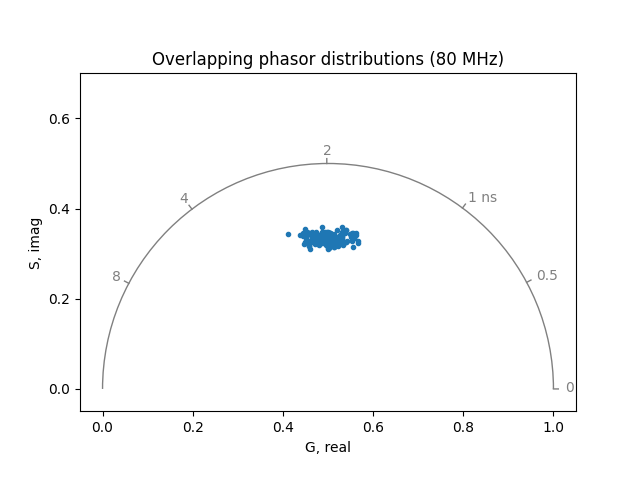
Overlapping phasor distributions#
The phasor coordinates of different multi-exponential decays may be overlapping, indistinguishable at a certain frequency:
frequency = [80, 160, 240, 320, 400]

# create two distributions of phasor coordinates overlapping at 80 MHz
real0, imag0 = phasor_from_lifetime(
    frequency,
    lifetime=distribution([0.5, 4.0]),
    fraction=distribution([0.4, 0.6]),
)
real1, imag1 = phasor_from_lifetime(
    frequency,
    lifetime=distribution([1.0, 8.0]),
    fraction=distribution([0.6, 0.4]),
)
# merge the two distributions
real = numpy.hstack([real0, real1])
imag = numpy.hstack([imag0, imag1])

plot = PhasorPlot(
    frequency=frequency[0],
    title=f'Overlapping phasor distributions ({frequency[0]} MHz)',
)
plot.plot(real[0], imag[0], '.')
plot.show()
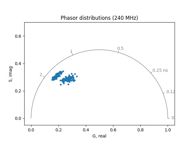
The distributions are better distinguishable at other frequencies:
plot = PhasorPlot(
    frequency=frequency[2],
    title=f'Phasor distributions ({frequency[2]} MHz)',
)
plot.plot(real[2], imag[2], '.')
plot.show()
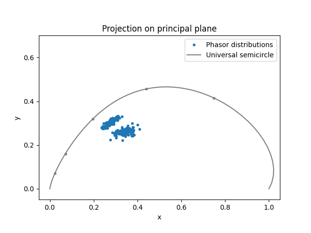
Project onto principal plane#
The projection of the multi-harmonic phasor coordinates onto the principal plane should give an overall good representation of the distribution.
The transformation matrix can be used to project other multi-harmonic phasor coordinates onto the same plane, for example the universal semicircle:
x0, y0, transformation_matrix = phasor_to_principal_plane(real, imag)

lifetimes, _ = phasor_to_apparent_lifetime(
    *phasor_semicircle(), frequency=frequency[0]
)
lifetimes[0] = 1e9
x1, y1 = numpy.dot(
    transformation_matrix,
    numpy.vstack(phasor_from_lifetime(frequency, lifetimes)),
)
x2, y2 = numpy.dot(
    transformation_matrix,
    numpy.vstack(phasor_from_lifetime(frequency, [0.5, 1.0, 2.0, 4.0, 8.0])),
)

plot = PhasorPlot(
    title='Projection on principal plane', grid=False, xlabel='x', ylabel='y'
)
plot.plot(x0, y0, '.', label='Phasor distributions')
plot.plot(x1, y1, '-', color='0.5', label='Universal semicircle')
plot.plot(x2, y2, '.', color='0.5')
plot.show()
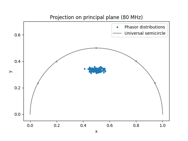
For single harmonic input, the projected, reoriented coordinates match the original, single harmonics phasor coordinates (compare to the first figure):
x0, y0, transformation_matrix = phasor_to_principal_plane(real[:1], imag[:1])
x1, y1 = numpy.dot(
    transformation_matrix,
    numpy.vstack(phasor_from_lifetime(frequency[0], lifetimes, keepdims=True)),
)
x2, y2 = numpy.dot(
    transformation_matrix,
    numpy.vstack(
        phasor_from_lifetime(
            frequency[0], [0.5, 1.0, 2.0, 4.0, 8.0], keepdims=True
        )
    ),
)

plot = PhasorPlot(
    title=f'Projection on principal plane ({frequency[0]} MHz)',
    grid=False,
    xlabel='x',
    ylabel='y',
)
plot.plot(x0, y0, '.', label='Phasor distributions')
plot.plot(x1, y1, '-', color='0.5', label='Universal semicircle')
plot.plot(x2, y2, '.', color='0.5')
plot.show()
TODO: demonstrate on real data that linearity is preserved and visualization by cursors is applicable.
sphinx_gallery_thumbnail_number = -2 mypy: allow-untyped-defs, allow-untyped-calls mypy: disable-error-code=”arg-type”
Total running time of the script: (0 minutes 0.194 seconds)