Component analysis#
An introduction to component analysis in phasor space.
Import required modules, functions, and classes:
import math

import matplotlib.animation as animation
import matplotlib.pyplot as plt
import numpy

from phasorpy.components import (
    graphical_component_analysis,
    two_fractions_from_phasor,
)
from phasorpy.phasor import phasor_from_lifetime
from phasorpy.plot import PhasorPlot

numpy.random.seed(42)
component_style = {
    'linestyle': '-',
    'marker': 'o',
    'color': 'tab:blue',
    'fontsize': 14,
}
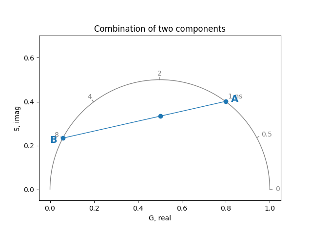
Fractions of two components#
The phasor coordinates of combinations of two lifetime components lie on the line between the two components. For example, a combination with 60% contribution (fraction 0.6) of a component A with lifetime 1.0 ns and 40% contribution (fraction 0.4) of a component B with lifetime 8.0 ns at 80 MHz:
frequency = 80.0
component_lifetimes = [1.0, 8.0]
component_fractions = [0.6, 0.4]

components_real, components_imag = phasor_from_lifetime(
    frequency, component_lifetimes
)

plot = PhasorPlot(frequency=frequency, title='Combination of two components')
plot.components(
    components_real,
    components_imag,
    component_fractions,
    labels=['A', 'B'],
    **component_style,
)
plot.show()
If the location of both components is known, their contributions (fractions) to the phasor point that lies on the line between the components can be calculated:
real, imag = phasor_from_lifetime(
    frequency, component_lifetimes, component_fractions
)

fraction_of_first_component = two_fractions_from_phasor(
    real, imag, components_real, components_imag
)

assert math.isclose(fraction_of_first_component, component_fractions[0])
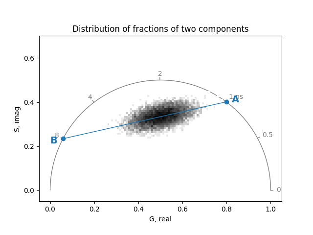
Distribution of fractions of two components#
Phasor coordinates can have different contributions of two components with known phasor coordinates:
real, imag = numpy.random.multivariate_normal(
    (real, imag), [[5e-3, 1e-3], [1e-3, 1e-3]], (100, 100)
).T

plot = PhasorPlot(
    frequency=frequency, title='Distribution of fractions of two components'
)
plot.hist2d(real, imag, cmap='Greys')
plot.components(
    components_real, components_imag, labels=['A', 'B'], **component_style
)
plot.show()
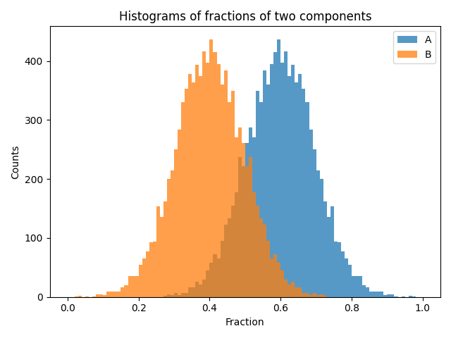
If the phasor coordinates of two components contributing to multiple phasor coordinates are known, their fractional contributions to each phasor coordinate can be calculated by projecting the phasor coordinate onto the line between the components. The fractions are plotted as histograms:
fraction_of_first_component = two_fractions_from_phasor(
    real, imag, components_real, components_imag
)

fig, ax = plt.subplots()
ax.hist(
    fraction_of_first_component.flatten(),
    range=(0, 1),
    bins=100,
    alpha=0.75,
    label='A',
)
ax.hist(
    1.0 - fraction_of_first_component.flatten(),
    range=(0, 1),
    bins=100,
    alpha=0.75,
    label='B',
)
ax.set_title('Histograms of fractions of two components')
ax.set_xlabel('Fraction')
ax.set_ylabel('Counts')
ax.legend()
plt.tight_layout()
plt.show()
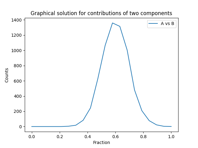
Graphical solution for contributions of two components#
The phasorpy.components.graphical_component_analysis()
function for two components counts the number of phasor coordinates
that fall within a radius at given fractions along the line between
the components.
Compare the plot of counts vs fraction to the previous histogram:
radius = 0.025
fractions = numpy.linspace(0.0, 1.0, 20)

counts = graphical_component_analysis(
    real,
    imag,
    components_real,
    components_imag,
    fractions=fractions,
    radius=radius,
)

fig, ax = plt.subplots()
ax.plot(fractions, counts[0], '-', label='A vs B')
ax.set_title('Graphical solution for contributions of two components')
ax.set_xlabel('Fraction')
ax.set_ylabel('Counts')
ax.legend()
plt.show()
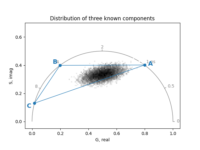
Graphical solution for contributions of three components#
The graphical solution can similarly be applied to the contributions of three components.
component_lifetimes = [1.0, 4.0, 15.0]
components_real, components_imag = phasor_from_lifetime(
    frequency, component_lifetimes
)

plot = PhasorPlot(
    frequency=frequency,
    title='Distribution of three known components',
)
plot.hist2d(real, imag, cmap='Greys')
plot.components(
    components_real, components_imag, labels=['A', 'B', 'C'], **component_style
)
plot.show()
The results of the graphical component analysis are plotted as histograms for each component pair:
counts = graphical_component_analysis(
    real,
    imag,
    components_real,
    components_imag,
    fractions=fractions,
    radius=radius,
)

fig, ax = plt.subplots()
ax.plot(fractions, counts[0], '-', label='A vs B')
ax.plot(fractions, counts[1], '-', label='A vs C')
ax.plot(fractions, counts[2], '-', label='B vs C')
ax.set_title('Graphical solution for contributions of three components')
ax.set_xlabel('Fraction')
ax.set_ylabel('Counts')
ax.legend()
plt.show()
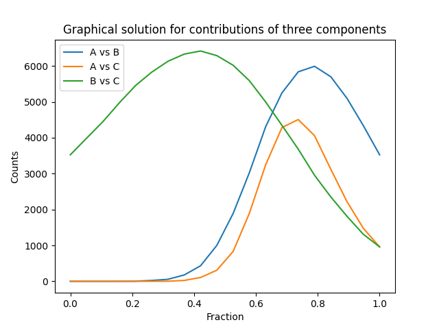
The graphical method for resolving the contribution of three components (pairwise) to a phasor coordinate is based on the quantification of moving circular cursors along the line between the components, demonstrated in the following animation for component A vs B. For the full analysis, the process is repeated for the other combinations of components, A vs C and B vs C:
fig, (ax, hist) = plt.subplots(nrows=2, ncols=1, figsize=(5.5, 8))

plot = PhasorPlot(
    frequency=frequency,
    ax=ax,
    title='Graphical solution for contribution of A vs B',
)
plot.hist2d(real, imag, cmap='Greys')
plot.components(
    components_real[:2],
    components_imag[:2],
    labels=['A', 'B'],
    **component_style,
)
plot.components(
    components_real[2], components_imag[2], labels=['C'], **component_style
)

hist.set_xlim(0, 1)
hist.set_xlabel('Fraction')
hist.set_ylabel('Counts')

direction_real = components_real[0] - components_real[1]
direction_imag = components_imag[0] - components_imag[1]

plots = []
for i in range(fractions.size):
    cursor_real = components_real[1] + fractions[i] * direction_real
    cursor_imag = components_imag[1] + fractions[i] * direction_imag
    plot_lines = plot.plot(
        [cursor_real, components_real[2]],
        [cursor_imag, components_imag[2]],
        '-',
        linewidth=plot.dataunit_to_point * radius * 2 + 5,
        solid_capstyle='round',
        color='red',
        alpha=0.5,
    )
    hist_artists = plt.plot(
        fractions[: i + 1], counts[0][: i + 1], linestyle='-', color='tab:blue'
    )
    plots.append(plot_lines + hist_artists)

_ = animation.ArtistAnimation(fig, plots, interval=100, blit=True)
plt.tight_layout()
plt.show()
sphinx_gallery_thumbnail_number = 5 mypy: allow-untyped-defs, allow-untyped-calls mypy: disable-error-code=”arg-type”
Total running time of the script: (0 minutes 5.567 seconds)