Introduction to PhasorPy

An introduction to using the PhasorPy library.

PhasorPy is an open-source Python library for the analysis of fluorescence lifetime and hyperspectral images using the Phasor approach.

Using the PhasorPy library requires familiarity with the phasor approach, image processing, array programming, and Python.

Install Python

An installation of Python version 3.10 or higher is required to use the PhasorPy library. Python is an easy to learn, powerful programming language. Python installers can be obtained from, for example, Python.org or Anaconda.com. Refer to the Python Tutorial for an introduction to Python.

Install PhasorPy

To download and install the PhasorPy library and all its dependencies from the Python Package Index (PyPI), run the following command on a command prompt, shell, or terminal:

python -m pip install -U "phasorpy[all]"

Note

The PhasorPy library is in its early stages of development and has not yet been released to PyPI.

The development version of PhasorPy can be installed instead from the latest source code on GitHub. This requires a C compiler, such as XCode, Visual Studio, or gcc, to be installed:

python -m pip install -U git+https://github.com/phasorpy/phasorpy.git

Update optional dependencies as needed:

python -m pip install -U lfdfiles sdtfile ptufile

Import phasorpy

Start the Python interpreter, import the phasorpy package, and print its version:

import phasorpy

print(phasorpy.__version__)

0.1.dev

Besides the PhasorPy library, the numpy and matplotlib libraries are used for array computing and plotting throughout this tutorial:

import numpy
import tifffile  # TODO: from phasorpy.io import read_ometiff
from matplotlib import pyplot

from phasorpy.datasets import fetch

Read signal from file

The phasorpy.io module provides functions to read time-resolved and hyperspectral image stacks and metadata from many file formats used in microscopy, for example PicoQuant PTU, OME-TIFF, Zeiss LSM, and files written by SimFCS software. However, any other means that yields image stacks in numpy-array compatible form can be used instead. Image stacks, which may have any number of dimensions, are referred to as signal in the PhasorPy library.

The phasorpy.datasets module provides access to various sample files. For example, an Imspector TIFF file from the FLUTE project containing a time-correlated single photon counting (TCSPC) histogram of a zebrafish embryo at day 3, acquired at 80 MHz:

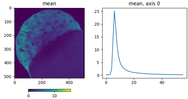
signal = tifffile.imread(fetch('Embryo.tif'))
frequency = 80.11  # MHz; from the XML metadata in the file

print(signal.shape, signal.dtype)

(56, 512, 512) uint16

Plot the spatial and histogram averages:

from phasorpy.plot import plot_signal_image

plot_signal_image(signal, axis=0)

Calculate phasor coordinates

The phasorpy.phasor module provides functions to calculate, calibrate, filter, and convert phasor coordinates.

Phasor coordinates are the real and imaginary components of the complex numbers returned by a real forward Digital Fourier Transform (DFT) of a signal at certain harmonics (multiples of the fundamental frequency), normalized by the mean intensity (the zeroth harmonic). Phasor coordinates are named real and imag in the PhasorPy library. In literature and other software, they are also known as \(G\) and \(S\) or \(a\) and \(b\) (as in \(a + bi\)).

Phasor coordinates of the first harmonic are calculated from the signal, a TCSPC histogram in this case. The histogram samples are in the first dimension (axis=0):

from phasorpy.phasor import phasor_from_signal

mean, real, imag = phasor_from_signal(signal, axis=0)

The phasor coordinates are undefined if the mean intensity is zero. In that case, the arrays contain special NaN (Not a Number) values, which are ignored in further analysis:

print(real[:4, :4])

[[        nan         nan -0.27292411         nan]
 [        nan         nan  0.16095963         nan]
 [        nan         nan  0.90096887         nan]
 [        nan  0.6234898          nan         nan]]

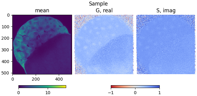
Plot the calculated phasor coordinates:

from phasorpy.plot import plot_phasor_image

plot_phasor_image(mean, real, imag, title='Sample')

By default, only the phasor coordinates at the first harmonic are calculated. However, only when the phasor coordinates at all harmonics are considered (including the mean intensity) is the signal completely described:

from phasorpy.phasor import phasor_to_signal

phasor_all_harmonics = phasor_from_signal(signal, axis=0, harmonic='all')
reconstructed_signal = phasor_to_signal(
    *phasor_all_harmonics, axis=0, samples=signal.shape[0]
)

numpy.testing.assert_allclose(
    numpy.nan_to_num(reconstructed_signal), signal, atol=1e-3
)

Calibrate phasor coordinates

The signals from time-resolved measurements are convoluted with an instrument response function, causing the phasor-coordinates to be phase-shifted and modulated (scaled) by unknown amounts. The phasor coordinates must therefore be calibrated with coordinates obtained from a reference standard of known lifetime, acquired with the same instrument settings.

In this case, a homogeneous solution of Fluorescein with a lifetime of 4.2 ns was imaged.

Read the signal of the reference measurement from a file:

reference_signal = tifffile.imread(fetch('Fluorescein_Embryo.tif'))

Calculate phasor coordinates from the measured reference signal:

reference_mean, reference_real, reference_imag = phasor_from_signal(
    reference_signal, axis=0
)

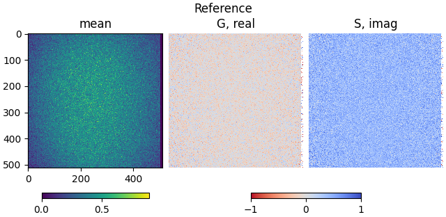
Show the calculated reference phasor coordinates:

plot_phasor_image(
    reference_mean, reference_real, reference_imag, title='Reference'
)

Calibrate the raw phasor coordinates with the reference coordinates of known lifetime (Fluorescein, 4.2 ns):

from phasorpy.phasor import phasor_calibrate

real, imag = phasor_calibrate(
    real,
    imag,
    reference_real,
    reference_imag,
    frequency=frequency,
    lifetime=4.2,
)

Show the calibrated phasor coordinates:

plot_phasor_image(mean, real, imag, title='Calibrated')

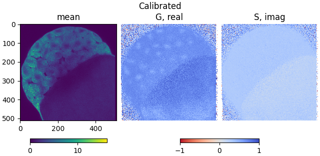
The phasor coordinates are now located in the first quadrant, except for some with low signal to noise level.

If necessary, the calibration can be undone/reversed using the same reference:

uncalibrated_real, uncalibrated_imag = phasor_calibrate(
    real,
    imag,
    reference_real,
    reference_imag,
    frequency=frequency,
    lifetime=4.2,
    reverse=True,
)

numpy.testing.assert_allclose(
    (mean, uncalibrated_real, uncalibrated_imag),
    phasor_from_signal(signal, axis=0),
    atol=1e-3,
)

Filter phasor coordinates

Applying median filter to the calibrated phasor coordinates, often multiple times, improves contrast and reduces noise:

from phasorpy.phasor import phasor_filter

real, imag = phasor_filter(real, imag, method='median', size=3, repeat=2)

Pixels with low intensities are commonly excluded from analysis and visualization of phasor coordinates:

from phasorpy.phasor import phasor_threshold

mean, real, imag = phasor_threshold(mean, real, imag, mean_min=1)

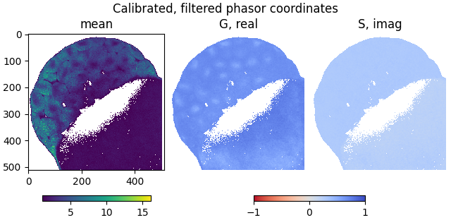
Show the calibrated, filtered phasor coordinates:

plot_phasor_image(
    mean, real, imag, title='Calibrated, filtered phasor coordinates'
)

Store phasor coordinates

Phasor coordinates and select metadata can be exported to OME-TIFF formatted files, which are compatible with Bio-Formats and Fiji.

Write the calibrated and filtered phasor coordinates, and frequency to an OME-TIFF file:

from phasorpy.io import phasor_from_ometiff, phasor_to_ometiff

phasor_to_ometiff(
    'phasors.ome.tif',
    mean,
    real,
    imag,
    frequency=frequency,
    harmonic=1,
    description=(
        'Phasor coordinates of a zebrafish embryo at day 3, '
        'calibrated, median-filtered, and thresholded.'
    ),
)

Read the phasor coordinates and metadata back from the OME-TIFF file:

mean_, real_, imag_, attrs = phasor_from_ometiff('phasors.ome.tif')

numpy.allclose(real_, real)
assert real_.dtype == numpy.float32
assert attrs['frequency'] == frequency
assert attrs['harmonic'] == 1
assert attrs['description'].startswith('Phasor coordinates of')

The functions also transparently work with multi-harmonic phasor coordinates.

Plot phasor coordinates

The phasorpy.plot module provides functions and classes for plotting phasor and polar coordinates.

Large number of phasor coordinates, such as obtained from imaging, are commonly visualized as 2D histograms:

from phasorpy.plot import PhasorPlot

phasorplot = PhasorPlot(
    frequency=frequency, title='Calibrated, filtered phasor coordinates'
)
phasorplot.hist2d(real, imag)
phasorplot.show()

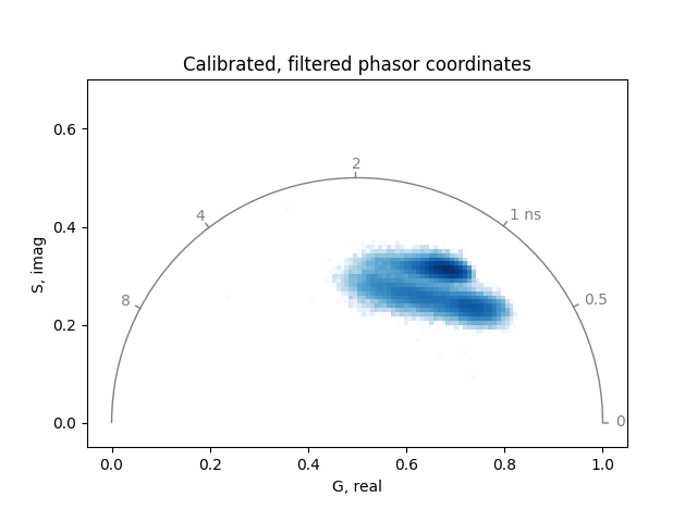
The calibrated phasor coordinates of all pixels lie inside the universal semicircle (on which theoretically the phasor coordinates of all single exponential lifetimes are located). That means, all pixels contain mixtures of signals from multiple lifetime components.

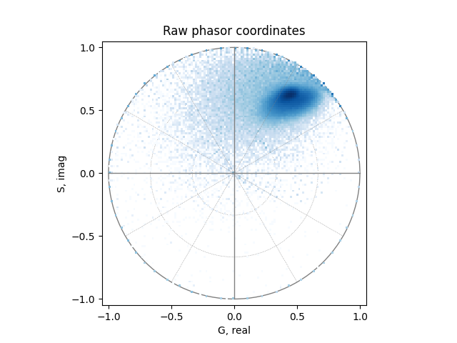
For comparison, the uncalibrated, unfiltered phasor coordinates:

phasorplot = PhasorPlot(allquadrants=True, title='Raw phasor coordinates')
phasorplot.hist2d(uncalibrated_real, uncalibrated_imag)
phasorplot.show()

Select phasor coordinates

# TODO

Component analysis

# TODO

Spectral phasors

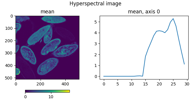
Phasor coordinates can be calculated from hyperspectral images (acquired at many equidistant emission wavelengths) and processed in much the same way as time-resolved signals. Calibration is not necessary.

Open a hyperspectral dataset acquired with a laser scanning microscope at 30 emission wavelengths:

from phasorpy.io import read_lsm

hyperspectral_signal = read_lsm(fetch('paramecium.lsm'))

plot_signal_image(hyperspectral_signal, axis=0, title='Hyperspectral image')

Calculate phasor coordinates at the first harmonic and filter out pixels with low intensities:

mean, real, imag = phasor_from_signal(hyperspectral_signal, axis=0)
_, real, imag = phasor_threshold(mean, real, imag, mean_min=1)

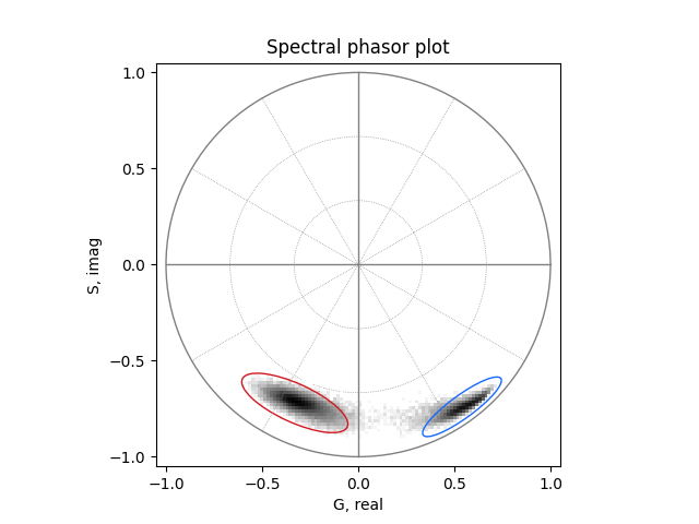
Plot the phasor coordinates as a two-dimensional histogram and select two clusters in the phasor plot by means of elliptical cursors:

from phasorpy.color import CATEGORICAL

cursors_real = [-0.33, 0.54]
cursors_imag = [-0.72, -0.74]
radius = [0.1, 0.06]
radius_minor = [0.3, 0.25]

phasorplot = PhasorPlot(allquadrants=True, title='Spectral phasor plot')
phasorplot.hist2d(real, imag, cmap='Greys')
for i in range(len(cursors_real)):
    phasorplot.cursor(
        cursors_real[i],
        cursors_imag[i],
        radius=radius[i],
        radius_minor=radius_minor[i],
        color=CATEGORICAL[i],
        linestyle='-',
    )
phasorplot.show()

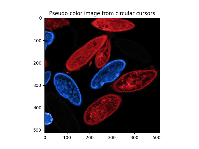
Use the elliptic cursors to mask regions of interest in the phasor space:

from phasorpy.cursors import mask_from_elliptic_cursor

elliptic_masks = mask_from_elliptic_cursor(
    real,
    imag,
    cursors_real,
    cursors_imag,
    radius=radius,
    radius_minor=radius_minor,
)

Plot a pseudo-color image, composited from the elliptic cursor masks and the mean intensity image:

from phasorpy.cursors import pseudo_color

pseudo_color_image = pseudo_color(*elliptic_masks, intensity=mean)

fig, ax = pyplot.subplots()
ax.set_title('Pseudo-color image from circular cursors')
ax.imshow(pseudo_color_image)
pyplot.show()

Appendix

Print information about Python interpreter and installed packages:

print(phasorpy.versions())

Python-3.12.5
phasorpy-0.1.dev
numpy-2.1.1
tifffile-2024.8.30
imagecodecs-n/a
lfdfiles-2024.9.15
sdtfile-2024.5.24
ptufile-2024.9.14
matplotlib-3.9.2
scipy-1.14.1
skimage-0.24.0
sklearn-n/a
pandas-2.2.2
xarray-2024.9.0
click-8.1.7
pooch-v1.8.2

sphinx_gallery_thumbnail_number = -5 mypy: allow-untyped-defs, allow-untyped-calls mypy: disable-error-code=”arg-type”