Phasor coordinates from lifetimes#
An introduction to the phasor_from_lifetime function.
The phasorpy.phasor.phasor_from_lifetime() function is used
to calculate phasor coordinates as a function of frequency,
single or multiple lifetime components, and the pre-exponential amplitudes
or fractional intensities of the components.
Import required modules and functions:
import numpy

from phasorpy.phasor import phasor_from_lifetime, phasor_to_polar
from phasorpy.plot import PhasorPlot, plot_phasor, plot_polar_frequency

rng = numpy.random.default_rng(42)
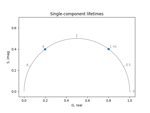
Single-component lifetimes#
The phasor coordinates of single-component lifetimes are located on the universal semicircle. For example, 4.0 ns and 1.0 ns at a frequency of 80 MHz:
frequency = 80.0
lifetimes = [4.0, 1.0]

plot_phasor(
    *phasor_from_lifetime(frequency, lifetimes),
    frequency=frequency,
    title='Single-component lifetimes',
)
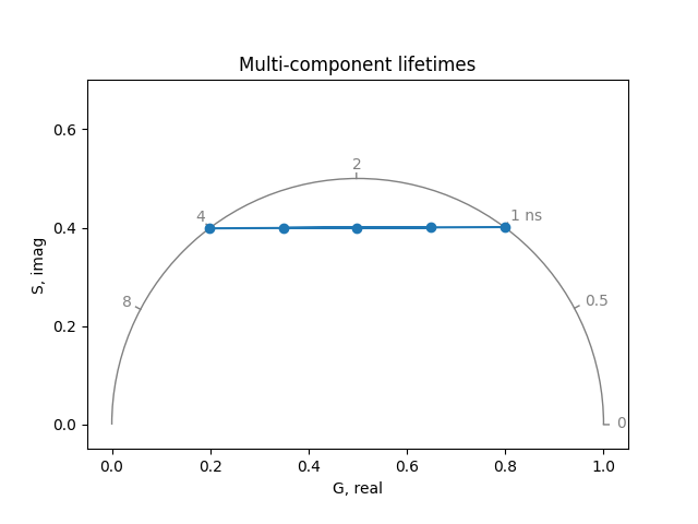
Multi-component lifetimes#
The phasor coordinates of two lifetime components with varying fractional intensities are linear combinations of the coordinates of the pure components:
fractions = numpy.array(
    [[1, 0], [0.25, 0.75], [0.5, 0.5], [0.75, 0.25], [0, 1]]
)

plot_phasor(
    *phasor_from_lifetime(frequency, lifetimes, fractions),
    linestyle='-',
    frequency=frequency,
    title='Multi-component lifetimes',
)
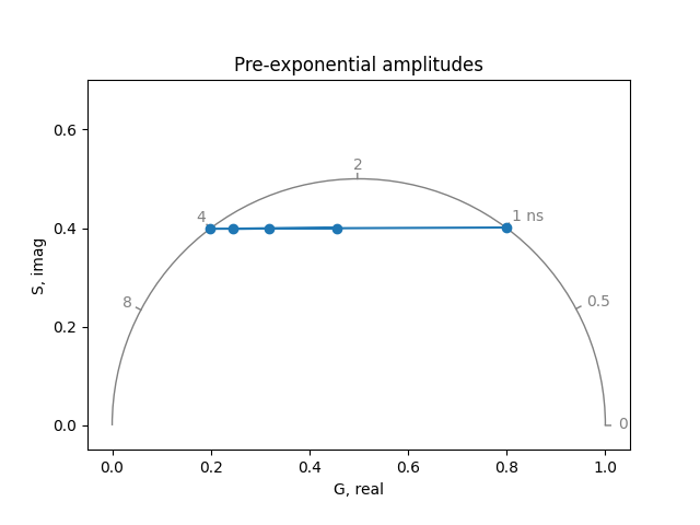
Pre-exponential amplitudes#
The phasor coordinates of two lifetime components with varying pre-exponential amplitudes are also located on a line:
plot_phasor(
    *phasor_from_lifetime(
        frequency, lifetimes, fractions, preexponential=True
    ),
    linestyle='-',
    frequency=frequency,
    title='Pre-exponential amplitudes',
)
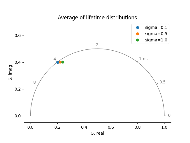
Average of lifetime distributions#
The average phasor coordinates for wider distributions of lifetimes lie further inside the universal semicircle compared to the narrower distributions:
frequency = 80.0
lifetime = 4.0
standard_deviations = [0.1, 0.5, 1.0]
samples = 100000

plot = PhasorPlot(
    frequency=frequency, title='Average of lifetime distributions'
)
for sigma in standard_deviations:
    phi = numpy.sqrt(sigma * sigma / lifetime)
    phasor_average = numpy.average(
        phasor_from_lifetime(
            frequency, rng.gamma(lifetime / phi, phi, samples)
        ),
        axis=1,
    )
    plot.plot(*phasor_average, label=f'{sigma=:.1f}')
plot.show()
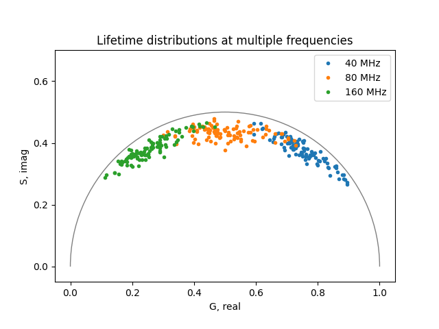
Lifetime distributions at multiple frequencies#
Phasor coordinates can be calculated at once for many frequencies, lifetime components, and their fractions. As an example, random distrinutions of lifetimes and their fractions are plotted at three frequencies. Lifetimes are passed in units of s and frequencies in Hz, requiring to specify a unit_conversion factor:
samples = 100
lifetimes = [4.0, 2.0, 1.0]

lifetime_distributions = (
    numpy.column_stack(
        [rng.gamma(lifetime / 0.01, 0.01, samples) for lifetime in lifetimes]
    )
    * 1e-9
)
fraction_distributions = numpy.column_stack(
    [rng.random(samples) for lifetime in lifetimes]
)

plot_phasor(
    *phasor_from_lifetime(
        frequency=[40e6, 80e6, 160e6],
        lifetime=lifetime_distributions,
        fraction=fraction_distributions,
        unit_conversion=1.0,
    ),
    marker='.',
    label=('40 MHz', '80 MHz', '160 MHz'),
    title='Lifetime distributions at multiple frequencies',
)
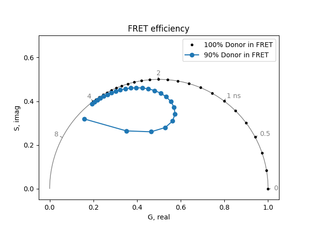
FRET efficiency#
The phasor coordinates of a fluorescence energy transfer donor with a single lifetime component of 4.0 ns as a function of FRET efficiency at a frequency of 80 MHz, with some background signal and about 90 % of the donors participating in energy transfer, are on a curved trajectory. For comparison, when 100% donors participate in FRET and there is no background signal, the phasor coordinates lie on the universal semicircle:
frequency = 80.0
samples = 25
lifetime = 4.0
efficiency = numpy.linspace(0.0, 1.0, samples)

lifetime_quenched = lifetime * (1.0 - efficiency)

plot = PhasorPlot(frequency=frequency, title='FRET efficiency')
plot.plot(
    *phasor_from_lifetime(frequency, lifetime_quenched),
    color='k',
    marker='.',
    label='100% Donor in FRET',
)
plot.plot(
    *phasor_from_lifetime(
        frequency,
        lifetime=numpy.column_stack(
            (
                numpy.full(samples, lifetime),  # donor-only lifetime
                lifetime_quenched,  # donor lifetime with FRET
                numpy.full(samples, 1e9),  # background with long lifetime
            )
        ),
        fraction=[0.1, 0.9, 0.1 / 1e9],
        preexponential=True,
    ),
    linestyle='-',
    label='90% Donor in FRET',
)
plot.show()
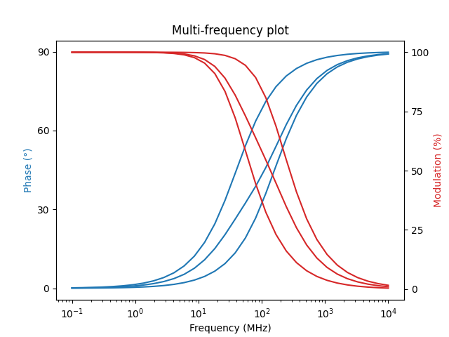
Multi-frequency plot#
Phase shift and demodulation of multi-component lifetimes can be calculated as a function of the excitation light frequency and fractional intensities:
frequencies = numpy.logspace(-1, 4, 32)
lifetimes = [4.0, 1.0]
fractions = numpy.array([[1, 0], [0.5, 0.5], [0, 1]])

plot_polar_frequency(
    frequencies,
    *phasor_to_polar(*phasor_from_lifetime(frequencies, lifetimes, fractions)),
    title='Multi-frequency plot',
)
sphinx_gallery_thumbnail_number = -2 mypy: allow-untyped-defs, allow-untyped-calls mypy: disable-error-code=”arg-type”
Total running time of the script: (0 minutes 0.470 seconds)